1.6. Scipy : high-level scientific computing¶

Authors: Gaël Varoquaux, Adrien Chauve, Andre Espaze, Emmanuelle Gouillart, Ralf Gommers

Scipy

The scipy package contains various toolboxes dedicated to common issues in scientific computing. Its different submodules correspond to different applications, such as interpolation, integration, optimization, image processing, statistics, special functions, etc.

Tip

scipy can be compared to other standard scientific-computing libraries, such as the GSL (GNU Scientific Library for C and C++), or Matlab’s toolboxes. scipy is the core package for scientific routines in Python; it is meant to operate efficiently on numpy arrays, so that numpy and scipy work hand in hand.

Before implementing a routine, it is worth checking if the desired data processing is not already implemented in Scipy. As non-professional programmers, scientists often tend to re-invent the wheel, which leads to buggy, non-optimal, difficult-to-share and unmaintainable code. By contrast, Scipy’s routines are optimized and tested, and should therefore be used when possible.

Chapters contents

Warning

This tutorial is far from an introduction to numerical computing. As enumerating the different submodules and functions in scipy would be very boring, we concentrate instead on a few examples to give a general idea of how to use scipy for scientific computing.

scipy is composed of task-specific sub-modules:

`scipy.cluster`	Vector quantization / Kmeans
`scipy.constants`	Physical and mathematical constants
`scipy.fftpack`	Fourier transform
`scipy.integrate`	Integration routines
`scipy.interpolate`	Interpolation
`scipy.io`	Data input and output
`scipy.linalg`	Linear algebra routines
`scipy.ndimage`	n-dimensional image package
`scipy.odr`	Orthogonal distance regression
`scipy.optimize`	Optimization
`scipy.signal`	Signal processing
`scipy.sparse`	Sparse matrices
`scipy.spatial`	Spatial data structures and algorithms
`scipy.special`	Any special mathematical functions
`scipy.stats`	Statistics

Tip

They all depend on numpy, but are mostly independent of each other. The standard way of importing Numpy and these Scipy modules is:

>>> importnumpyasnp
>>> fromscipyimportstats# same for other sub-modules

The main scipy namespace mostly contains functions that are really numpy functions (try scipy.cos is np.cos). Those are exposed for historical reasons; there’s no reason to use import scipy in your code.

1.6.1. File input/output: `scipy.io`¶

Matlab files: Loading and saving:

>>> fromscipyimportioasspio
>>> a=np.ones((3,3))
>>> spio.savemat('file.mat',{'a':a})# savemat expects a dictionary
>>> data=spio.loadmat('file.mat')
>>> data['a']
array([[1.,  1.,  1.],
       [1.,  1.,  1.],
       [1.,  1.,  1.]])

Warning

Python / Matlab mismatches, eg matlab does not represent 1D arrays

>>> a=np.ones(3)
>>> a
array([1.,  1.,  1.])
>>> spio.savemat('file.mat',{'a':a})
>>> spio.loadmat('file.mat')['a']
array([[1.,  1.,  1.]])

Notice the difference?

Image files: Reading images:

>>> importimageio
>>> imageio.imread('fname.png')
Array(...)
>>> # Matplotlib also has a similar function
>>> importmatplotlib.pyplotasplt
>>> plt.imread('fname.png')
array(...)

See also

Load text files: numpy.loadtxt()/numpy.savetxt()
Clever loading of text/csv files: numpy.genfromtxt()/numpy.recfromcsv()
Fast and efficient, but numpy-specific, binary format: numpy.save()/numpy.load()
More advanced input/output of images in scikit-image: skimage.io

1.6.2. Special functions: `scipy.special`¶

Special functions are transcendental functions. The docstring of the scipy.special module is well-written, so we won’t list all functions here. Frequently used ones are:

Bessel function, such as scipy.special.jn() (nth integer order Bessel function)

Elliptic function (scipy.special.ellipj() for the Jacobian elliptic function, …)

Gamma function: scipy.special.gamma(), also note scipy.special.gammaln() which will give the log of Gamma to a higher numerical precision.

Erf, the area under a Gaussian curve: scipy.special.erf()

1.6.3. Linear algebra operations: `scipy.linalg`¶

Tip

The scipy.linalg module provides standard linear algebra operations, relying on an underlying efficient implementation (BLAS, LAPACK).

The scipy.linalg.det() function computes the determinant of a square matrix:

>>> fromscipyimportlinalg
>>> arr=np.array([[1,2],
... [3,4]])
>>> linalg.det(arr)
-2.0
>>> arr=np.array([[3,2],
... [6,4]])
>>> linalg.det(arr)
0.0
>>> linalg.det(np.ones((3,4)))
Traceback (most recent call last):
...
ValueError: expected square matrix

The scipy.linalg.inv() function computes the inverse of a square matrix:

>>> arr=np.array([[1,2],
... [3,4]])
>>> iarr=linalg.inv(arr)
>>> iarr
array([[-2. ,  1. ],
       [ 1.5, -0.5]])
>>> np.allclose(np.dot(arr,iarr),np.eye(2))
True

Finally computing the inverse of a singular matrix (its determinant is zero) will raise LinAlgError:

>>> arr=np.array([[3,2],
... [6,4]])
>>> linalg.inv(arr)
Traceback (most recent call last):
...
...LinAlgError: singular matrix

More advanced operations are available, for example singular-value decomposition (SVD):
```
>>> arr = np.arange(9).reshape((3, 3)) + np.diag([1, 0, 1])
>>> uarr, spec, vharr = linalg.svd(arr)
```
The resulting array spectrum is:
```
>>> spec    
array([14.88982544,   0.45294236,   0.29654967])
```
The original matrix can be re-composed by matrix multiplication of the outputs of svd with np.dot:
```
>>> sarr = np.diag(spec)
>>> svd_mat = uarr.dot(sarr).dot(vharr)
>>> np.allclose(svd_mat, arr)
True
```
SVD is commonly used in statistics and signal processing. Many other standard decompositions (QR, LU, Cholesky, Schur), as well as solvers for linear systems, are available in scipy.linalg.

1.6.4. Interpolation: `scipy.interpolate`¶

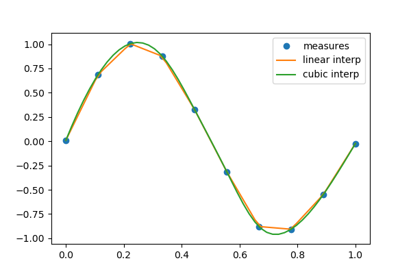
scipy.interpolate is useful for fitting a function from experimental data and thus evaluating points where no measure exists. The module is based on the FITPACK Fortran subroutines.

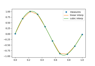
By imagining experimental data close to a sine function:

>>> measured_time=np.linspace(0,1,10)
>>> noise=(np.random.random(10)*2-1)*1e-1
>>> measures=np.sin(2*np.pi*measured_time)+noise

scipy.interpolate.interp1d can build a linear interpolation function:

>>> fromscipy.interpolateimportinterp1d
>>> linear_interp=interp1d(measured_time,measures)

../_images/sphx_glr_plot_interpolation_001.png

Then the result can be evaluated at the time of interest:

>>> interpolation_time=np.linspace(0,1,50)
>>> linear_results=linear_interp(interpolation_time)

A cubic interpolation can also be selected by providing the kind optional keyword argument:

>>> cubic_interp=interp1d(measured_time,measures,kind='cubic')
>>> cubic_results=cubic_interp(interpolation_time)

scipy.interpolate.interp2d is similar to scipy.interpolate.interp1d, but for 2-D arrays. Note that for the interp family, the interpolation points must stay within the range of given data points. See the summary exercise on Maximum wind speed prediction at the Sprogø station for a more advanced spline interpolation example.

1.6.5. Optimization and fit: `scipy.optimize`¶

Optimization is the problem of finding a numerical solution to a minimization or equality.

Tip

The scipy.optimize module provides algorithms for function minimization (scalar or multi-dimensional), curve fitting and root finding.

>>> fromscipyimportoptimize

1.6.5.1. Curve fitting¶

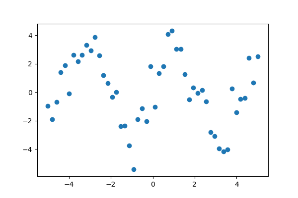
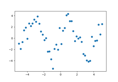
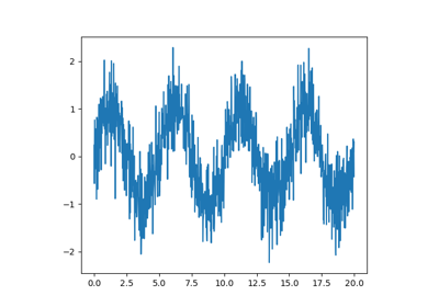
../_images/sphx_glr_plot_curve_fit_001.png

Suppose we have data on a sine wave, with some noise:

>>> x_data=np.linspace(-5,5,num=50)
>>> y_data=2.9*np.sin(1.5*x_data)+np.random.normal(size=50)

If we know that the data lies on a sine wave, but not the amplitudes or the period, we can find those by least squares curve fitting. First we have to define the test function to fit, here a sine with unknown amplitude and period:

>>> deftest_func(x,a,b):
... returna*np.sin(b*x)

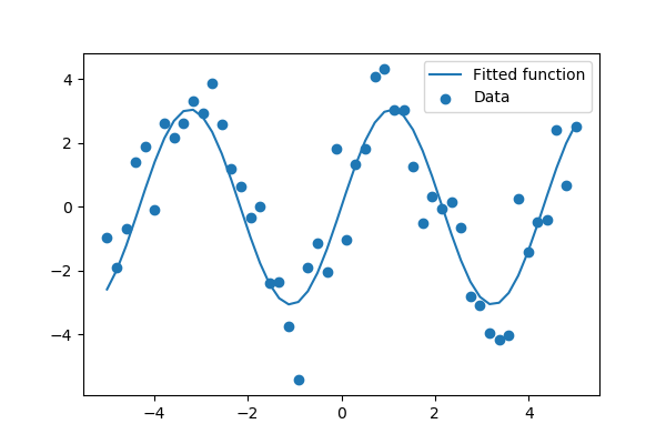
../_images/sphx_glr_plot_curve_fit_002.png

We then use scipy.optimize.curve_fit() to find $a$ and $b$ :

>>> params,params_covariance=optimize.curve_fit(test_func,x_data,y_data,p0=[2,2])
>>> print(params)
[3.05931973  1.45754553]

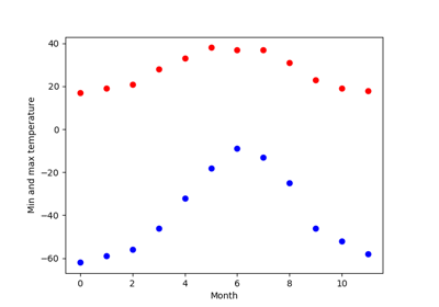
Exercise: Curve fitting of temperature data

The temperature extremes in Alaska for each month, starting in January, are given by (in degrees Celcius):
max:  17,  19,  21,  28,  33,  38, 37,  37,  31,  23,  19,  18
min: -62, -59, -56, -46, -32, -18, -9, -13, -25, -46, -52, -58
Plot these temperature extremes.

Define a function that can describe min and max temperatures. Hint: this function has to have a period of 1 year. Hint: include a time offset.

Fit this function to the data with scipy.optimize.curve_fit().

Plot the result. Is the fit reasonable? If not, why?

Is the time offset for min and max temperatures the same within the fit accuracy?

solution

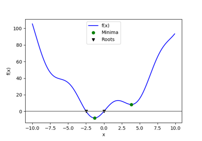
1.6.5.2. Finding the minimum of a scalar function¶

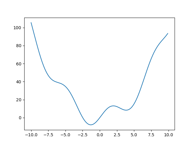
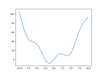
../_images/sphx_glr_plot_optimize_example1_001.png

Let’s define the following function:

>>> deff(x):
... returnx**2+10*np.sin(x)

and plot it:

>>> x=np.arange(-10,10,0.1)
>>> plt.plot(x,f(x))
>>> plt.show()

This function has a global minimum around -1.3 and a local minimum around 3.8.

Searching for minimum can be done with scipy.optimize.minimize(), given a starting point x0, it returns the location of the minimum that it has found:

>>> result=optimize.minimize(f,x0=0)
>>> result
      fun: -7.9458233756...
 hess_inv: array([[0.0858...]])
      jac: array([-1.19209...e-06])
  message: 'Optimization terminated successfully.'
     nfev: 18
      nit: 5
     njev: 6
   status: 0
  success: True
        x: array([-1.30644...])
>>> result.x# The coordinate of the minimum  
array([-1.30644...])

Methods: As the function is a smooth function, gradient-descent based methods are good options. The lBFGS algorithm is a good choice in general:

>>> optimize.minimize(f,x0=0,method="L-BFGS-B")
      fun: array([-7.94582338])
 hess_inv: <1x1 LbfgsInvHessProduct with dtype=float64>
      jac: array([-1.42108547e-06])
  message: ...'CONVERGENCE: NORM_OF_PROJECTED_GRADIENT_<=_PGTOL'
     nfev: 12
      nit: 5
   status: 0
  success: True
        x: array([-1.30644013])

Note how it cost only 12 functions evaluation above to find a good value for the minimum.

Global minimum: A possible issue with this approach is that, if the function has local minima, the algorithm may find these local minima instead of the global minimum depending on the initial point x0:

>>> res=optimize.minimize(f,x0=3,method="L-BFGS-B")
>>> res.x
array([3.83746709])

If we don’t know the neighborhood of the global minimum to choose the initial point, we need to resort to costlier global optimization. To find the global minimum, we use scipy.optimize.basinhopping() (added in version 0.12.0 of Scipy). It combines a local optimizer with sampling of starting points:

>>> optimize.basinhopping(f,0)
                  nfev: 1725
 minimization_failures: 0
                   fun: -7.9458233756152845
                     x: array([-1.30644001])
               message: ['requested number of basinhopping iterations completed successfully']
                  njev: 575
                   nit: 100

Note

scipy used to contain the routine anneal, it has been removed in SciPy 0.16.0.

Constraints: We can constrain the variable to the interval (0, 10) using the “bounds” argument:

>>> res=optimize.minimize(f,x0=1,
... bounds=((0,10),))
>>> res.x
array([0.])

Tip

What has happened? Why are we finding 0, which is not a mimimum of our function.

Minimizing functions of several variables

To minimize over several variables, the trick is to turn them into a function of a multi-dimensional variable (a vector). See for instance the exercise on 2D minimization below.

Note

scipy.optimize.minimize_scalar() is a function with dedicated methods to minimize functions of only one variable.

See also

Finding minima of function is discussed in more details in the advanced chapter: Mathematical optimization: finding minima of functions.

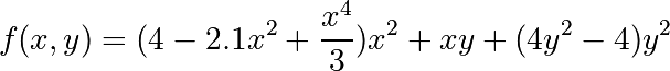
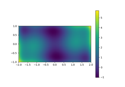
Exercise: 2-D minimization

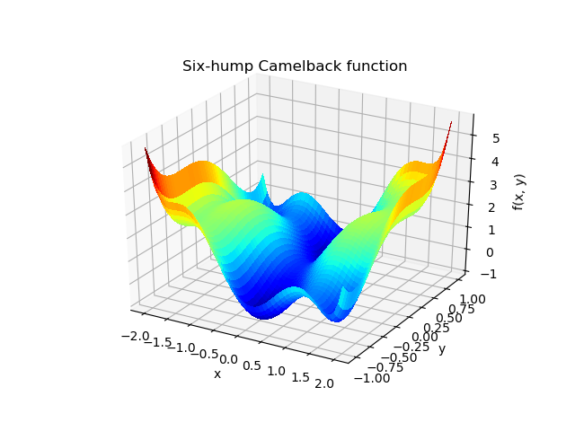
The six-hump camelback function

$f(x, y) = (4 - 2.1x^2 + \frac{x^4}{3})x^2 + xy + (4y^2 - 4)y^2$

has multiple global and local minima. Find the global minima of this function.

Hints:

Variables can be restricted to $-2 < x < 2$ and $-1 < y < 1$ .

Use numpy.meshgrid() and matplotlib.pyplot.imshow() to find visually the regions.

Use scipy.optimize.minimize(), optionally trying out several of its methods.

How many global minima are there, and what is the function value at those points? What happens for an initial guess of $(x, y) = (0, 0)$ ?

solution

1.6.5.3. Finding the roots of a scalar function¶

To find a root, i.e. a point where $f(x) = 0$ , of the function $f$ above we can use scipy.optimize.root():

>>> root=optimize.root(f,x0=1)# our initial guess is 1
>>> root# The full result
    fjac: array([[-1.]])
     fun: array([0.])
 message: 'The solution converged.'
    nfev: 10
     qtf: array([1.33310463e-32])
       r: array([-10.])
  status: 1
 success: True
       x: array([0.])
>>> root.x# Only the root found
array([0.])

Note that only one root is found. Inspecting the plot of $f$ reveals that there is a second root around -2.5. We find the exact value of it by adjusting our initial guess:

>>> root2=optimize.root(f,x0=-2.5)
>>> root2.x
array([-2.47948183])

Note

scipy.optimize.root() also comes with a variety of algorithms, set via the “method” argument.

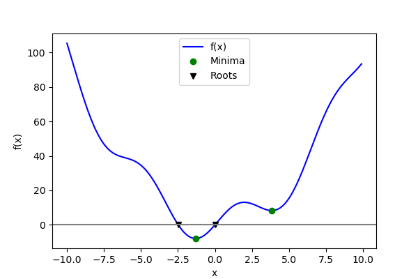
../_images/sphx_glr_plot_optimize_example2_001.png

Now that we have found the minima and roots of f and used curve fitting on it, we put all those results together in a single plot:

See also

You can find all algorithms and functions with similar functionalities in the documentation of scipy.optimize.

See the summary exercise on Non linear least squares curve fitting: application to point extraction in topographical lidar data for another, more advanced example.

1.6.6. Statistics and random numbers: `scipy.stats`¶

The module scipy.stats contains statistical tools and probabilistic descriptions of random processes. Random number generators for various random process can be found in numpy.random.

1.6.6.1. Distributions: histogram and probability density function¶

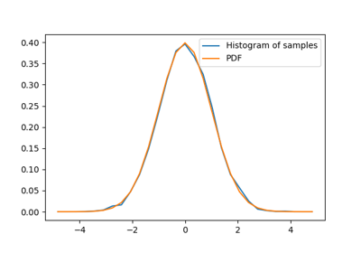
Given observations of a random process, their histogram is an estimator of the random process’s PDF (probability density function):

>>> samples=np.random.normal(size=1000)
>>> bins=np.arange(-4,5)
>>> bins
array([-4, -3, -2, -1,  0,  1,  2,  3,  4])
>>> histogram=np.histogram(samples,bins=bins,density=True)[0]
>>> bins=0.5*(bins[1:]+bins[:-1])
>>> bins
array([-3.5, -2.5, -1.5, -0.5,  0.5,  1.5,  2.5,  3.5])
>>> fromscipyimportstats
>>> pdf=stats.norm.pdf(bins)# norm is a distribution object
>>> plt.plot(bins,histogram)
[<matplotlib.lines.Line2D object at ...>]
>>> plt.plot(bins,pdf)
[<matplotlib.lines.Line2D object at ...>]

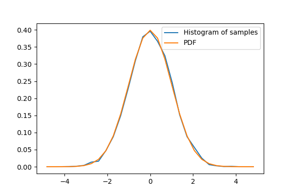
../_images/sphx_glr_plot_normal_distribution_001.png

If we know that the random process belongs to a given family of random processes, such as normal processes, we can do a maximum-likelihood fit of the observations to estimate the parameters of the underlying distribution. Here we fit a normal process to the observed data:

>>> loc,std=stats.norm.fit(samples)
>>> loc
-0.045256707...
>>> std
0.9870331586...

Exercise: Probability distributions

Generate 1000 random variates from a gamma distribution with a shape parameter of 1, then plot a histogram from those samples. Can you plot the pdf on top (it should match)?

Extra: the distributions have many useful methods. Explore them by reading the docstring or by using tab completion. Can you recover the shape parameter 1 by using the fit method on your random variates?

1.6.6.2. Mean, median and percentiles¶

The mean is an estimator of the center of the distribution:

>>> np.mean(samples)
-0.0452567074...

The median another estimator of the center. It is the value with half of the observations below, and half above:

>>> np.median(samples)
-0.0580280347...

Tip

Unlike the mean, the median is not sensitive to the tails of the distribution. It is “robust”.

Exercise: Compare mean and median on samples of a Gamma distribution

Which one seems to be the best estimator of the center for the Gamma distribution?

The median is also the percentile 50, because 50% of the observation are below it:

>>> stats.scoreatpercentile(samples,50)
-0.0580280347...

Similarly, we can calculate the percentile 90:

>>> stats.scoreatpercentile(samples,90)
1.2315935511...

Tip

The percentile is an estimator of the CDF: cumulative distribution function.

1.6.6.3. Statistical tests¶

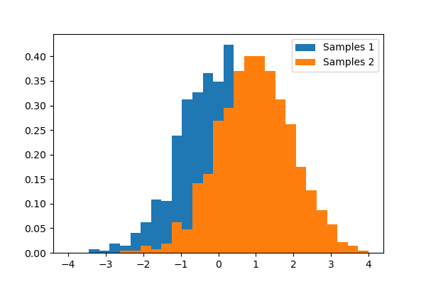
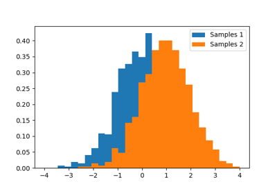
A statistical test is a decision indicator. For instance, if we have two sets of observations, that we assume are generated from Gaussian processes, we can use a T-test to decide whether the means of two sets of observations are significantly different:

>>> a=np.random.normal(0,1,size=100)
>>> b=np.random.normal(1,1,size=10)
>>> stats.ttest_ind(a,b)
(array(-3.177574054...), 0.0019370639...)

Tip

The resulting output is composed of:

The T statistic value: it is a number the sign of which is proportional to the difference between the two random processes and the magnitude is related to the significance of this difference.
the p value: the probability of both processes being identical. If it is close to 1, the two process are almost certainly identical. The closer it is to zero, the more likely it is that the processes have different means.

See also

The chapter on statistics introduces much more elaborate tools for statistical testing and statistical data loading and visualization outside of scipy.

1.6.7. Numerical integration: `scipy.integrate`¶

1.6.7.1. Function integrals¶

The most generic integration routine is scipy.integrate.quad(). To compute $\int_0^{\pi / 2} sin(t) dt$ :

>>> fromscipy.integrateimportquad
>>> res,err=quad(np.sin,0,np.pi/2)
>>> np.allclose(res,1)# res is the result, is should be close to 1
True
>>> np.allclose(err,1-res)# err is an estimate of the err
True

Other integration schemes are available: scipy.integrate.fixed_quad(), scipy.integrate.quadrature(), scipy.integrate.romberg()…

1.6.7.2. Integrating differential equations¶

scipy.integrate also features routines for integrating Ordinary Differential Equations (ODE). In particular, scipy.integrate.odeint() solves ODE of the form:

dy/dt=rhs(y1,y2,..,t0,...)

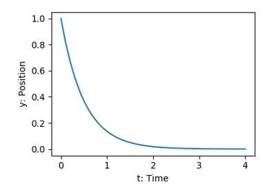
As an introduction, let us solve the ODE $\frac{dy}{dt} = -2 y$ between $t = 0 \dots 4$ , with the initial condition $y(t=0) = 1$ . First the function computing the derivative of the position needs to be defined:

>>> defcalc_derivative(ypos,time):
... return-2*ypos

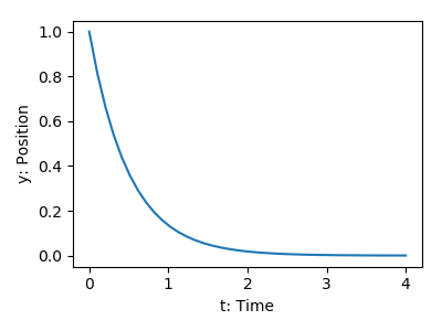
../_images/sphx_glr_plot_odeint_simple_001.png

Then, to compute y as a function of time:

>>> fromscipy.integrateimportodeint
>>> time_vec=np.linspace(0,4,40)
>>> y=odeint(calc_derivative,y0=1,t=time_vec)

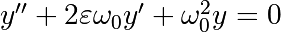
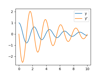
Let us integrate a more complex ODE: a damped spring-mass oscillator. The position of a mass attached to a spring obeys the 2nd order ODE $y'' + 2 \varepsilon \omega_0 y' + \omega_0^2 y = 0$ with $\omega_0^2 = k/m$ with $k$ the spring constant, $m$ the mass and $\varepsilon = c/(2 m \omega_0)$ with $c$ the damping coefficient. We set:

>>> mass=0.5# kg
>>> kspring=4# N/m
>>> cviscous=0.4# N s/m

Hence:

>>> eps=cviscous/(2*mass*np.sqrt(kspring/mass))
>>> omega=np.sqrt(kspring/mass)

The system is underdamped, as:

>>> eps<1
True

For odeint(), the 2nd order equation needs to be transformed in a system of two first-order equations for the vector $Y = (y, y')$ : the function computes the velocity and acceleration:

>>> defcalc_deri(yvec,time,eps,omega):
... return(yvec[1],-2.0*eps*omega*yvec[1]-omega**2*yvec[0])

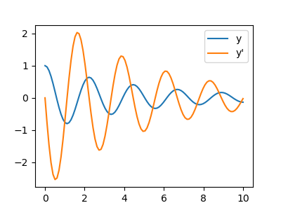
../_images/sphx_glr_plot_odeint_damped_spring_mass_001.png

Integration of the system follows:

>>> time_vec=np.linspace(0,10,100)
>>> yinit=(1,0)
>>> yarr=odeint(calc_deri,yinit,time_vec,args=(eps,omega))

Tip

scipy.integrate.odeint() uses the LSODA (Livermore Solver for Ordinary Differential equations with Automatic method switching for stiff and non-stiff problems), see the ODEPACK Fortran library for more details.

See also

Partial Differental Equations

There is no Partial Differential Equations (PDE) solver in Scipy. Some Python packages for solving PDE’s are available, such as fipy or SfePy.

1.6.8. Fast Fourier transforms: `scipy.fftpack`¶

The scipy.fftpack module computes fast Fourier transforms (FFTs) and offers utilities to handle them. The main functions are:

scipy.fftpack.fft() to compute the FFT
scipy.fftpack.fftfreq() to generate the sampling frequencies
scipy.fftpack.ifft() computes the inverse FFT, from frequency space to signal space

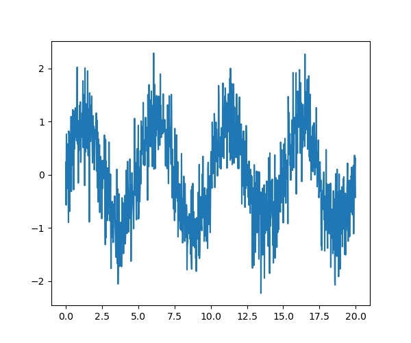
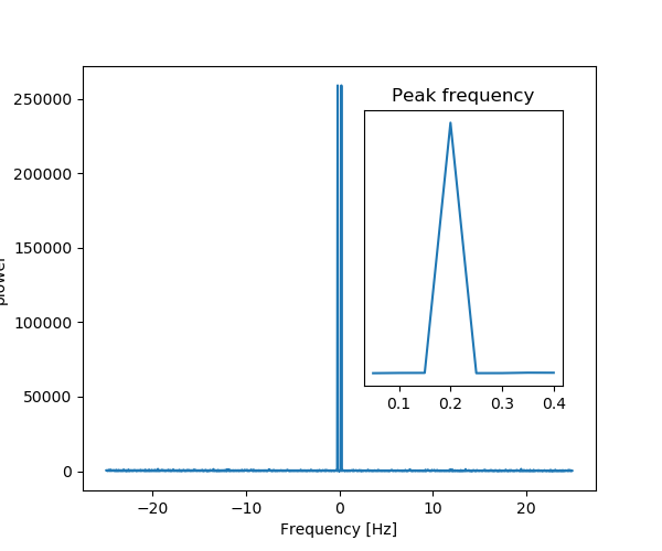
As an illustration, a (noisy) input signal (sig), and its FFT:

>>> fromscipyimportfftpack
>>> sig_fft=fftpack.fft(sig)
>>> freqs=fftpack.fftfreq(sig.size,d=time_step)


Signal	FFT

As the signal comes from a real function, the Fourier transform is symmetric.

The peak signal frequency can be found with freqs[power.argmax()]

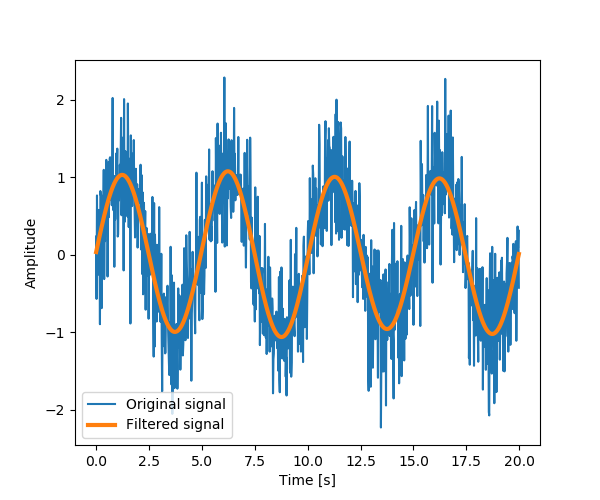
../_images/sphx_glr_plot_fftpack_003.png

Setting the Fourrier component above this frequency to zero and inverting the FFT with scipy.fftpack.ifft(), gives a filtered signal.

Note

The code of this example can be found here

numpy.fft

Numpy also has an implementation of FFT (numpy.fft). However, the scipy one should be preferred, as it uses more efficient underlying implementations.

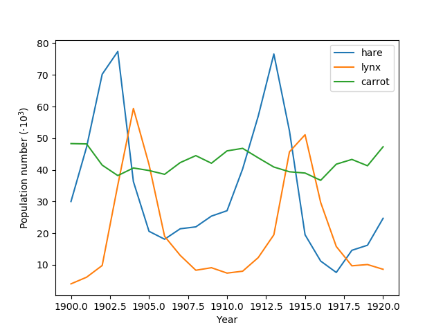
Fully worked examples:

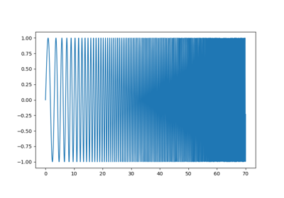
Crude periodicity finding (link)	Gaussian image blur (link)

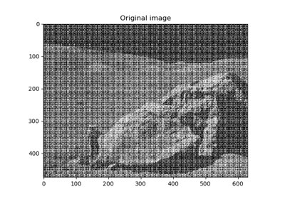
Exercise: Denoise moon landing image

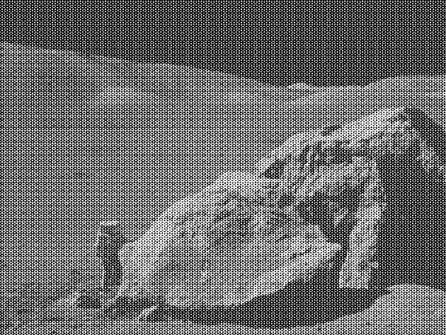
Examine the provided image moonlanding.png, which is heavily contaminated with periodic noise. In this exercise, we aim to clean up the noise using the Fast Fourier Transform.
Load the image using matplotlib.pyplot.imread().
Find and use the 2-D FFT function in scipy.fftpack, and plot the spectrum (Fourier transform of) the image. Do you have any trouble visualising the spectrum? If so, why?
The spectrum consists of high and low frequency components. The noise is contained in the high-frequency part of the spectrum, so set some of those components to zero (use array slicing).
Apply the inverse Fourier transform to see the resulting image.

Solution

1.6.9. Signal processing: `scipy.signal`¶

Tip

scipy.signal is for typical signal processing: 1D, regularly-sampled signals.

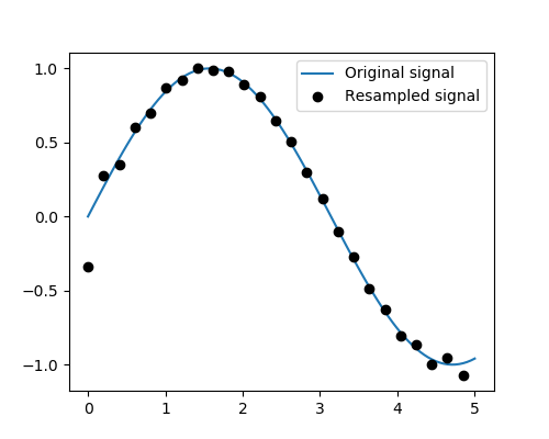
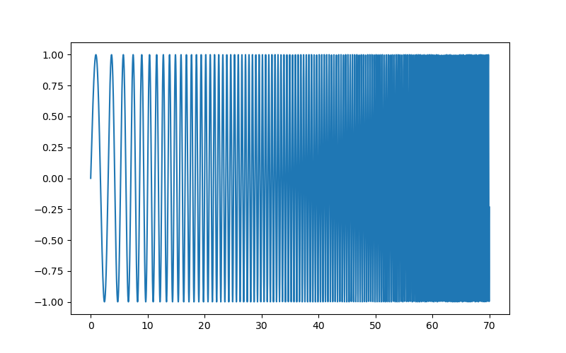
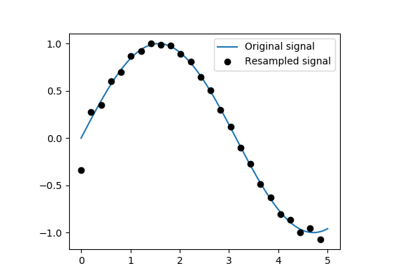
../_images/sphx_glr_plot_resample_001.png

Resampling scipy.signal.resample(): resample a signal to n points using FFT.

>>> t=np.linspace(0,5,100)
>>> x=np.sin(t)
>>> fromscipyimportsignal
>>> x_resampled=signal.resample(x,25)
>>> plt.plot(t,x)
[<matplotlib.lines.Line2D object at ...>]
>>> plt.plot(t[::4],x_resampled,'ko')
[<matplotlib.lines.Line2D object at ...>]

Tip

Notice how on the side of the window the resampling is less accurate and has a rippling effect.

This resampling is different from the interpolation provided by scipy.interpolate as it only applies to regularly sampled data.

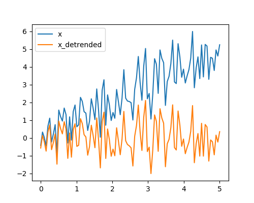
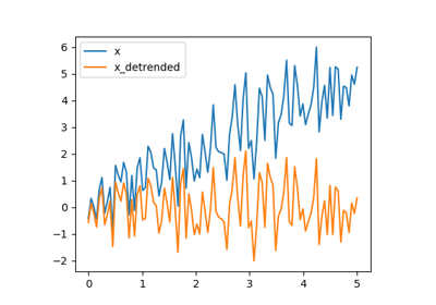
../_images/sphx_glr_plot_detrend_001.png

Detrending scipy.signal.detrend(): remove linear trend from signal:

>>> t=np.linspace(0,5,100)
>>> x=t+np.random.normal(size=100)
>>> fromscipyimportsignal
>>> x_detrended=signal.detrend(x)
>>> plt.plot(t,x)
[<matplotlib.lines.Line2D object at ...>]
>>> plt.plot(t,x_detrended)
[<matplotlib.lines.Line2D object at ...>]

Filtering: For non-linear filtering, scipy.signal has filtering (median filter scipy.signal.medfilt(), Wiener scipy.signal.wiener()), but we will discuss this in the image section.

Tip

scipy.signal also has a full-blown set of tools for the design of linear filter (finite and infinite response filters), but this is out of the scope of this tutorial.

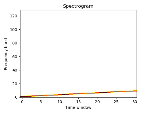
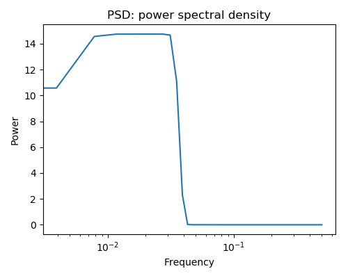
Spectral analysis: scipy.signal.spectrogram() compute a spectrogram –frequency spectrums over consecutive time windows–, while scipy.signal.welch() comptes a power spectrum density (PSD).

1.6.10. Image manipulation: `scipy.ndimage`¶

scipy.ndimage provides manipulation of n-dimensional arrays as images.

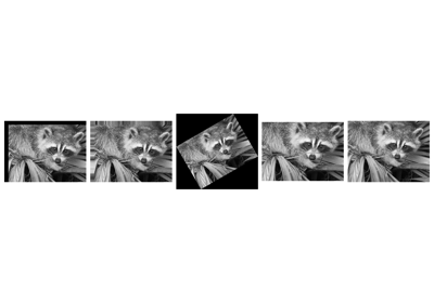
1.6.10.1. Geometrical transformations on images¶

Changing orientation, resolution, ..

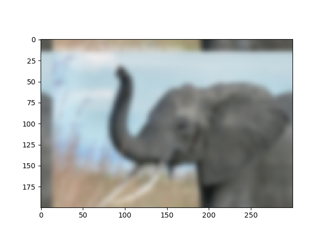
>>> fromscipyimportmisc# Load an image
>>> face=misc.face(gray=True)
>>> fromscipyimportndimage# Shift, roate and zoom it
>>> shifted_face=ndimage.shift(face,(50,50))
>>> shifted_face2=ndimage.shift(face,(50,50),mode='nearest')
>>> rotated_face=ndimage.rotate(face,30)
>>> cropped_face=face[50:-50,50:-50]
>>> zoomed_face=ndimage.zoom(face,2)
>>> zoomed_face.shape
(1536, 2048)

../_images/sphx_glr_plot_image_transform_001.png

>>> plt.subplot(151)
<matplotlib.axes._subplots.AxesSubplot object at 0x...>
>>> plt.imshow(shifted_face,cmap=plt.cm.gray)
<matplotlib.image.AxesImage object at 0x...>
>>> plt.axis('off')
(-0.5, 1023.5, 767.5, -0.5)
>>> # etc.

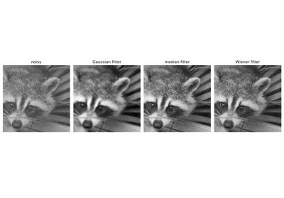
1.6.10.2. Image filtering¶

Generate a noisy face:

>>> fromscipyimportmisc
>>> face=misc.face(gray=True)
>>> face=face[:512,-512:]# crop out square on right
>>> importnumpyasnp
>>> noisy_face=np.copy(face).astype(np.float)
>>> noisy_face+=face.std()*0.5*np.random.standard_normal(face.shape)

Apply a variety of filters on it:

>>> blurred_face=ndimage.gaussian_filter(noisy_face,sigma=3)
>>> median_face=ndimage.median_filter(noisy_face,size=5)
>>> fromscipyimportsignal
>>> wiener_face=signal.wiener(noisy_face,(5,5))

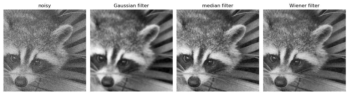
../_images/sphx_glr_plot_image_filters_001.png

Other filters in scipy.ndimage.filters and scipy.signal can be applied to images.

Exercise

Compare histograms for the different filtered images.

1.6.10.3. Mathematical morphology¶

Tip

Mathematical morphology stems from set theory. It characterizes and transforms geometrical structures. Binary (black and white) images, in particular, can be transformed using this theory: the sets to be transformed are the sets of neighboring non-zero-valued pixels. The theory was also extended to gray-valued images.

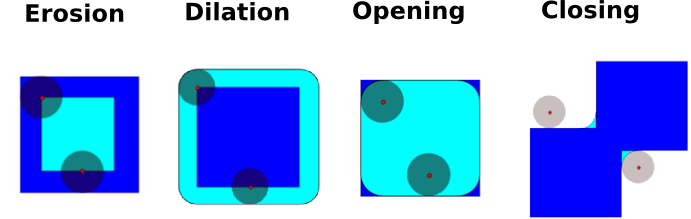
Mathematical-morphology operations use a structuring element in order to modify geometrical structures.

Let us first generate a structuring element:

>>> el=ndimage.generate_binary_structure(2,1)
>>> el
array([[False, True, False],
       [...True, True, True],
       [False, True, False]])
>>> el.astype(np.int)
array([[0, 1, 0],
       [1, 1, 1],
       [0, 1, 0]])

Erosion scipy.ndimage.binary_erosion()

>>> a=np.zeros((7,7),dtype=np.int)
>>> a[1:6,2:5]=1
>>> a
array([[0, 0, 0, 0, 0, 0, 0],
       [0, 0, 1, 1, 1, 0, 0],
       [0, 0, 1, 1, 1, 0, 0],
       [0, 0, 1, 1, 1, 0, 0],
       [0, 0, 1, 1, 1, 0, 0],
       [0, 0, 1, 1, 1, 0, 0],
       [0, 0, 0, 0, 0, 0, 0]])
>>> ndimage.binary_erosion(a).astype(a.dtype)
array([[0, 0, 0, 0, 0, 0, 0],
       [0, 0, 0, 0, 0, 0, 0],
       [0, 0, 0, 1, 0, 0, 0],
       [0, 0, 0, 1, 0, 0, 0],
       [0, 0, 0, 1, 0, 0, 0],
       [0, 0, 0, 0, 0, 0, 0],
       [0, 0, 0, 0, 0, 0, 0]])
>>> #Erosion removes objects smaller than the structure
>>> ndimage.binary_erosion(a,structure=np.ones((5,5))).astype(a.dtype)
array([[0, 0, 0, 0, 0, 0, 0],
       [0, 0, 0, 0, 0, 0, 0],
       [0, 0, 0, 0, 0, 0, 0],
       [0, 0, 0, 0, 0, 0, 0],
       [0, 0, 0, 0, 0, 0, 0],
       [0, 0, 0, 0, 0, 0, 0],
       [0, 0, 0, 0, 0, 0, 0]])

Dilation scipy.ndimage.binary_dilation()

>>> a=np.zeros((5,5))
>>> a[2,2]=1
>>> a
array([[0.,  0.,  0.,  0.,  0.],
       [0.,  0.,  0.,  0.,  0.],
       [0.,  0.,  1.,  0.,  0.],
       [0.,  0.,  0.,  0.,  0.],
       [0.,  0.,  0.,  0.,  0.]])
>>> ndimage.binary_dilation(a).astype(a.dtype)
array([[0.,  0.,  0.,  0.,  0.],
       [0.,  0.,  1.,  0.,  0.],
       [0.,  1.,  1.,  1.,  0.],
       [0.,  0.,  1.,  0.,  0.],
       [0.,  0.,  0.,  0.,  0.]])

Opening scipy.ndimage.binary_opening()

>>> a=np.zeros((5,5),dtype=np.int)
>>> a[1:4,1:4]=1
>>> a[4,4]=1
>>> a
array([[0, 0, 0, 0, 0],
       [0, 1, 1, 1, 0],
       [0, 1, 1, 1, 0],
       [0, 1, 1, 1, 0],
       [0, 0, 0, 0, 1]])
>>> # Opening removes small objects
>>> ndimage.binary_opening(a,structure=np.ones((3,3))).astype(np.int)
array([[0, 0, 0, 0, 0],
       [0, 1, 1, 1, 0],
       [0, 1, 1, 1, 0],
       [0, 1, 1, 1, 0],
       [0, 0, 0, 0, 0]])
>>> # Opening can also smooth corners
>>> ndimage.binary_opening(a).astype(np.int)
array([[0, 0, 0, 0, 0],
       [0, 0, 1, 0, 0],
       [0, 1, 1, 1, 0],
       [0, 0, 1, 0, 0],
       [0, 0, 0, 0, 0]])

Closing: scipy.ndimage.binary_closing()

Exercise

Check that opening amounts to eroding, then dilating.

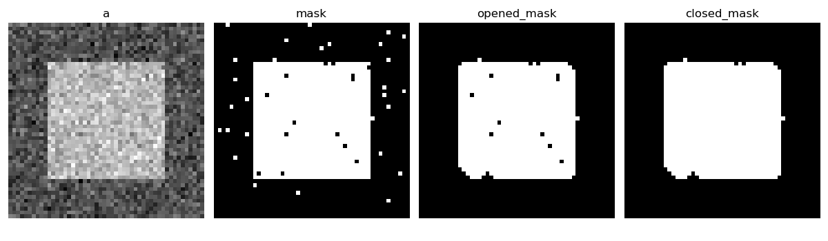
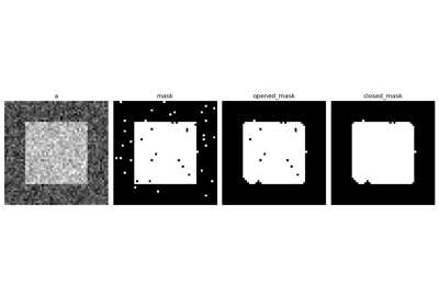
An opening operation removes small structures, while a closing operation fills small holes. Such operations can therefore be used to “clean” an image.

>>> a=np.zeros((50,50))
>>> a[10:-10,10:-10]=1
>>> a+=0.25*np.random.standard_normal(a.shape)
>>> mask=a>=0.5
>>> opened_mask=ndimage.binary_opening(mask)
>>> closed_mask=ndimage.binary_closing(opened_mask)

../_images/sphx_glr_plot_mathematical_morpho_001.png

Exercise

Check that the area of the reconstructed square is smaller than the area of the initial square. (The opposite would occur if the closing step was performed before the opening).

For gray-valued images, eroding (resp. dilating) amounts to replacing a pixel by the minimal (resp. maximal) value among pixels covered by the structuring element centered on the pixel of interest.

>>> a=np.zeros((7,7),dtype=np.int)
>>> a[1:6,1:6]=3
>>> a[4,4]=2;a[2,3]=1
>>> a
array([[0, 0, 0, 0, 0, 0, 0],
       [0, 3, 3, 3, 3, 3, 0],
       [0, 3, 3, 1, 3, 3, 0],
       [0, 3, 3, 3, 3, 3, 0],
       [0, 3, 3, 3, 2, 3, 0],
       [0, 3, 3, 3, 3, 3, 0],
       [0, 0, 0, 0, 0, 0, 0]])
>>> ndimage.grey_erosion(a,size=(3,3))
array([[0, 0, 0, 0, 0, 0, 0],
       [0, 0, 0, 0, 0, 0, 0],
       [0, 0, 1, 1, 1, 0, 0],
       [0, 0, 1, 1, 1, 0, 0],
       [0, 0, 3, 2, 2, 0, 0],
       [0, 0, 0, 0, 0, 0, 0],
       [0, 0, 0, 0, 0, 0, 0]])

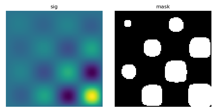
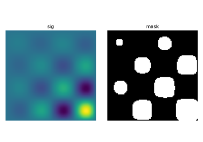
1.6.10.4. Connected components and measurements on images¶

Let us first generate a nice synthetic binary image.

>>> x,y=np.indices((100,100))
>>> sig=np.sin(2*np.pi*x/50.)*np.sin(2*np.pi*y/50.)*(1+x*y/50.**2)**2
>>> mask=sig>1

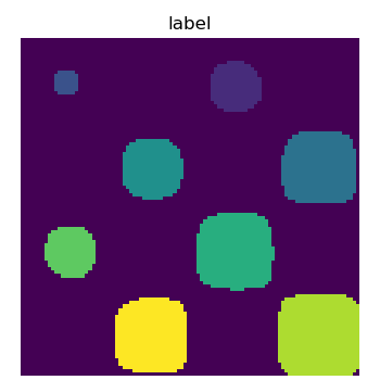
../_images/sphx_glr_plot_connect_measurements_001.png

../_images/sphx_glr_plot_connect_measurements_002.png

scipy.ndimage.label() assigns a different label to each connected component:

>>> labels,nb=ndimage.label(mask)
>>> nb
8

Now compute measurements on each connected component:

>>> areas=ndimage.sum(mask,labels,range(1,labels.max()+1))
>>> areas# The number of pixels in each connected component
array([190.,   45.,  424.,  278.,  459.,  190.,  549.,  424.])
>>> maxima=ndimage.maximum(sig,labels,range(1,labels.max()+1))
>>> maxima# The maximum signal in each connected component
array([ 1.80238238,   1.13527605,   5.51954079,   2.49611818, 6.71673619,
        1.80238238,  16.76547217,   5.51954079])

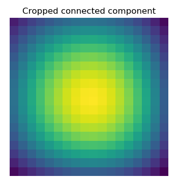
../_images/sphx_glr_plot_connect_measurements_003.png

Extract the 4th connected component, and crop the array around it:

>>> ndimage.find_objects(labels==4)
[(slice(30L, 48L, None), slice(30L, 48L, None))]
>>> sl=ndimage.find_objects(labels==4)
>>> frommatplotlibimportpyplotasplt
>>> plt.imshow(sig[sl[0]])
<matplotlib.image.AxesImage object at ...>

See the summary exercise on Image processing application: counting bubbles and unmolten grains for a more advanced example.

1.6.11. Summary exercises on scientific computing ¶

The summary exercises use mainly Numpy, Scipy and Matplotlib. They provide some real-life examples of scientific computing with Python. Now that the basics of working with Numpy and Scipy have been introduced, the interested user is invited to try these exercises.

Exercises:

Proposed solutions:

1.6.11.4. Example of solution for the image processing exercise: unmolten grains in glass

1.6.12. Full code examples for the scipy chapter ¶

Finding the minimum of a smooth function

Detrending a signal

Resample a signal with scipy.signal.resample

Integrating a simple ODE

Comparing 2 sets of samples from Gaussians

Integrate the Damped spring-mass oscillator

Normal distribution: histogram and PDF

Curve fitting

Spectrogram, power spectral density

A demo of 1D interpolation

Demo mathematical morphology

Plot geometrical transformations on images

Demo connected components

Minima and roots of a function

Plot filtering on images

Optimization of a two-parameter function

Plotting and manipulating FFTs for filtering

1.6.12.18. Solutions of the exercises for scipy¶

Crude periodicity finding

Curve fitting: temperature as a function of month of the year

Simple image blur by convolution with a Gaussian kernel

Image denoising by FFT

Gallery generated by Sphinx-Gallery

See also

References to go further

Some chapters of the advanced and the packages and applications parts of the scipy lectures
The scipy cookbook

1.6. Scipy : high-level scientific computing¶

1.6.1. File input/output: `scipy.io`¶

1.6.2. Special functions: `scipy.special`¶

1.6.3. Linear algebra operations: `scipy.linalg`¶

1.6.4. Interpolation: `scipy.interpolate`¶

1.6.5. Optimization and fit: `scipy.optimize`¶

1.6.5.1. Curve fitting¶

1.6.5.2. Finding the minimum of a scalar function¶

1.6.5.3. Finding the roots of a scalar function¶

1.6.6. Statistics and random numbers: `scipy.stats`¶

1.6.6.1. Distributions: histogram and probability density function¶

1.6.6.2. Mean, median and percentiles¶

1.6.6.3. Statistical tests¶

1.6.7. Numerical integration: `scipy.integrate`¶

1.6.7.1. Function integrals¶

1.6.7.2. Integrating differential equations¶

1.6.8. Fast Fourier transforms: `scipy.fftpack`¶

1.6.9. Signal processing: `scipy.signal`¶

1.6.10. Image manipulation: `scipy.ndimage`¶

1.6.10.1. Geometrical transformations on images¶

1.6.10.2. Image filtering¶

1.6.10.3. Mathematical morphology¶

1.6.10.4. Connected components and measurements on images¶

1.6.11. Summary exercises on scientific computing ¶

1.6.12. Full code examples for the scipy chapter ¶

1.6.12.18. Solutions of the exercises for scipy¶

Table Of Contents

Previous topic

Next topic

This Page